In the rapidly evolving landscape of artificial intelligence, the demand for computational efficiency and scalability has never been greater. While frameworks like TensorFlow and PyTorch have long dominated the scene, a powerful contender from Google’s research labs, JAX, is fundamentally changing how developers approach high-performance numerical computing and machine learning. JAX combines a familiar NumPy-like API with a potent set of function transformations—just-in-time (JIT) compilation, automatic differentiation, and parallelization—to unlock unprecedented performance on modern accelerators like GPUs and TPUs.

This article provides a comprehensive technical exploration of JAX, moving from its core principles to practical implementation and advanced techniques. We will delve into what makes JAX a go-to choice for cutting-edge research, particularly for the massive models that generate headlines in Google DeepMind News and OpenAI News. Whether you are a researcher aiming to scale novel architectures or an engineer looking to optimize complex numerical pipelines, understanding JAX is becoming an essential skill. We’ll explore its unique functional programming paradigm, demonstrate its power with practical code examples, and situate it within the broader ecosystem of tools like Flax, Optax, and the platforms discussed in AWS SageMaker News and Azure AI News.

The Four Pillars of JAX: Understanding jit, grad, vmap, and pmap

JAX’s power stems from a set of composable function transformations that operate on pure Python functions. These “pillars” allow you to write simple, Pythonic code that JAX transforms into highly optimized, hardware-accelerated computations. Understanding these four core functions—jit, grad, vmap, and pmap—is the key to unlocking JAX’s full potential.

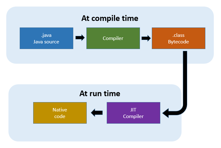
jit: Just-In-Time Compilation with XLA

The jit transformation is JAX’s secret weapon for performance. It uses Google’s Accelerated Linear Algebra (XLA) compiler to trace a Python function, convert it into an intermediate representation, and then compile it into highly optimized machine code specific to your hardware (CPU, GPU, or TPU). This process happens “just-in-time” when the function is first called. The result is that subsequent calls execute the fast, compiled version, often yielding speedups of 10-100x over native Python. This performance is critical for training the large models often discussed in Meta AI News and Mistral AI News.

Consider a simple function that computes a prediction using a set of learned weights. In plain NumPy, each operation is executed sequentially. With @jit, JAX can fuse these operations into a single, efficient kernel.

import jax
import jax.numpy as jnp
from jax import random, jit

# Generate some random data
key = random.PRNGKey(0)
X = random.normal(key, (1000, 100))
w = random.normal(key, (100, 1))
b = 0.5

# Define a simple linear prediction function
def predict(weights, bias, inputs):
    return jnp.dot(inputs, weights) + bias

# Compile the function with jit
jit_predict = jit(predict)

# First call compiles the function (and may be slower)
y_jit = jit_predict(w, b, X).block_until_ready()

# Subsequent calls are much faster
# In a real application, you would use %timeit in a notebook
# to measure the performance difference.
print("JIT-compiled function executed successfully.")

grad: Powerful and Flexible Automatic Differentiation

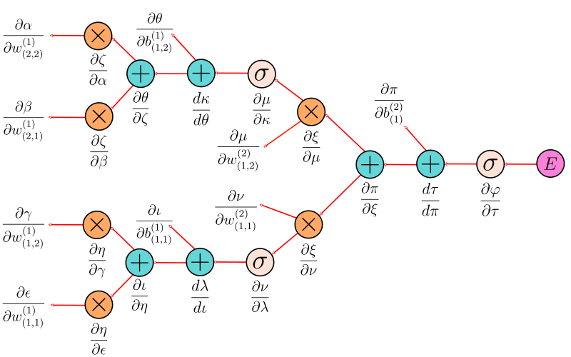
At the heart of modern machine learning is gradient-based optimization. JAX provides an incredibly flexible automatic differentiation system through its grad transformation. Unlike the tape-based autograd systems found in PyTorch or TensorFlow, JAX’s grad works by transforming a function that computes a value into a new function that computes its gradient. It can differentiate through a large subset of Python’s features, including loops, branches, and recursion, making it exceptionally powerful for research and complex model architectures.

Here’s how you can compute the gradient of a simple loss function with respect to its first argument (the parameters).

import jax
import jax.numpy as jnp
from jax import grad

# Define a simple squared error loss function
# Note: JAX's grad differentiates with respect to the first argument by default.
def squared_error_loss(params, x, y_true):
    y_pred = params['w'] * x + params['b']
    error = y_pred - y_true
    return jnp.mean(error**2)

# Initialize some parameters
params = {'w': 2.5, 'b': 0.8}
x_sample = 2.0
y_sample = 7.0

# Create a function that computes the gradient of the loss
grad_fn = grad(squared_error_loss)

# Calculate the gradients
gradients = grad_fn(params, x_sample, y_sample)

print(f"Gradients: {gradients}")
# Output will be a dictionary with gradients for 'w' and 'b'

vmap and pmap: Automatic Vectorization and Parallelization

vmap (vectorizing map) is a transformation that makes batching trivial. Instead of rewriting your function to handle an extra batch dimension, you can write it for a single example and then use vmap to automatically create a batched version. This keeps code clean and readable. pmap (parallel map) takes this a step further, allowing you to parallelize computations across multiple devices, such as the multiple GPUs in a server, a key topic in NVIDIA AI News.

Building a Neural Network with JAX and Flax

While JAX provides the low-level primitives, building and managing complex neural networks requires a higher-level framework. JAX’s functional nature means that functions cannot have internal state or side effects. This is a departure from the object-oriented approach of PyTorch’s nn.Module or Keras layers. Libraries like Flax (from Google) and Haiku (from DeepMind) provide elegant solutions for managing model parameters and state within this functional paradigm.

The Challenge of State in a Functional World

In JAX, all data, including model parameters, must be passed explicitly as arguments to functions. A function like a training step takes the current parameters as input and returns the *new, updated* parameters as output. This purity is what enables JAX’s powerful transformations but requires a different way of thinking. Flax helps structure this by separating the model definition (the architecture) from the state (the parameters).

Defining and Training a Model with Flax

Flax uses a module system that feels familiar but operates functionally. You define your network architecture by subclassing `flax.linen.Module`. The parameters are not stored within the module instance (`self.params`) but are initialized separately and passed to the module’s `apply` method during the forward pass.

Here is how you can define a simple Multi-Layer Perceptron (MLP), initialize its parameters, and define a JIT-compiled training step. This workflow is the foundation for training everything from simple classifiers to the complex models featured in Hugging Face Transformers News.

import jax
import jax.numpy as jnp
from jax import random, jit, grad
from flax import linen as nn
import optax # A popular optimization library for JAX

# 1. Define the model architecture using Flax
class SimpleMLP(nn.Module):
    features: list[int]

    @nn.compact
    def __call__(self, x):
        for feat in self.features[:-1]:
            x = nn.relu(nn.Dense(features=feat)(x))
        x = nn.Dense(features=self.features[-1])(x)
        return x

# 2. Initialize model parameters and optimizer state
key = random.PRNGKey(42)
dummy_input = jnp.ones((1, 128)) # Batch size 1, 128 features
model = SimpleMLP(features=[256, 128, 10]) # Example: 10 output classes
params = model.init(key, dummy_input)['params']
optimizer = optax.adam(learning_rate=1e-3)
opt_state = optimizer.init(params)

# 3. Define the loss function
def loss_fn(params, batch_inputs, batch_labels):
    logits = model.apply({'params': params}, batch_inputs)
    one_hot_labels = jax.nn.one_hot(batch_labels, num_classes=10)
    loss = optax.softmax_cross_entropy(logits, one_hot_labels).mean()
    return loss

# 4. Define a JIT-compiled training step
@jit
def train_step(params, opt_state, batch_inputs, batch_labels):
    # Calculate loss and gradients
    loss_val, grads = jax.value_and_grad(loss_fn)(params, batch_inputs, batch_labels)
    
    # Update parameters and optimizer state
    updates, new_opt_state = optimizer.update(grads, opt_state, params)
    new_params = optax.apply_updates(params, updates)
    
    return new_params, new_opt_state, loss_val

# Example usage (in a real training loop)
# new_params, new_opt_state, loss = train_step(params, opt_state, inputs, labels)
print("Flax model and train step defined successfully.")
print(f"Parameter shapes: {jax.tree_util.tree_map(lambda x: x.shape, params)}")

This pattern of creating a `train_step` function and compiling it with `@jit` is central to writing efficient JAX code. It ensures that the entire process of forward pass, loss calculation, backpropagation, and optimizer update is fused into a single, highly optimized kernel by XLA. Experiment tracking for such a process can be managed using tools from the MLflow News or Weights & Biases News ecosystems.

Advanced Techniques: Scaling with pmap and the JAX Ecosystem

JAX truly shines when scaling up to large models and massive datasets, a domain often covered by Kaggle News and cloud platform updates like Vertex AI News. The `pmap` transformation is the primary tool for this, enabling seamless data parallelism across multiple devices.

Multi-Device Training with `pmap`

pmap works similarly to `vmap`, but instead of mapping over a new batch axis, it maps over devices. When you apply `pmap` to a function, JAX compiles and runs a version of that function on each available device. Data is automatically split and distributed across these devices along the first axis. For a training step, this means each GPU or TPU core processes a unique shard of the data batch. Crucially, you must handle gradient aggregation manually using collective operations like `jax.lax.pmean` to average the gradients across all devices before applying the optimizer update.

The following example shows how to adapt our `train_step` for multi-GPU training.

import jax
import jax.numpy as jnp
from flax.training import train_state
import optax

# (Assuming SimpleMLP model and params are defined as before)

# Create a TrainState to bundle params, optimizer state, etc.
# This is a common pattern in Flax applications.
state = train_state.TrainState.create(
    apply_fn=model.apply,
    params=params,
    tx=optax.adam(1e-3),
)

# Define the training step for a single device
def single_device_train_step(state, batch):
    inputs, labels = batch
    
    def loss_fn(params):
        logits = state.apply_fn({'params': params}, inputs)
        one_hot_labels = jax.nn.one_hot(labels, num_classes=10)
        loss = optax.softmax_cross_entropy(logits, one_hot_labels).mean()
        return loss, logits

    grad_fn = jax.value_and_grad(loss_fn, has_aux=True)
    (loss, logits), grads = grad_fn(state.params)
    
    # Crucial step for pmap: average gradients across all devices
    grads = jax.lax.pmean(grads, axis_name='devices')
    
    # Apply updates
    state = state.apply_gradients(grads=grads)
    return state, loss

# Create the parallel training step with pmap
# The axis_name 'devices' is used to identify the axis for collectives.
p_train_step = jax.pmap(single_device_train_step, axis_name='devices')

# In a real scenario:
# 1. Replicate the initial state across all devices
#    p_state = jax.device_put_replicated(state, jax.local_devices())
# 2. Reshape data so the first dimension is num_devices
#    num_devices = jax.local_device_count()
#    batch_size = 32
#    global_batch_size = batch_size * num_devices
#    # ... reshape your data ...
# 3. Call the parallel step
#    p_state, p_loss = p_train_step(p_state, sharded_batch)

print("Parallel train step with pmap defined successfully.")

This approach forms the basis of large-scale training efforts seen from companies like Anthropic News and Cohere News. For deployment, models trained in JAX can be exported to standard formats like those discussed in ONNX News and served via high-performance engines like the Triton Inference Server News reports on.

Best Practices, Pitfalls, and Optimization

Working effectively with JAX requires embracing its functional paradigm and being mindful of how its transformations work. Here are some key best practices and common pitfalls to avoid.

Embrace Pure Functions

JAX transformations like jit and grad assume that your functions are “pure.” A pure function’s output depends only on its inputs, and it has no side effects (like modifying a global variable or printing to the console). Violating this can lead to unexpected behavior because JAX may cache results or trace the function only once. Always pass state explicitly and return updated state as an output.

Avoid Data-Dependent Python Control Flow

A common pitfall for beginners is using standard Python control flow (like an `if` statement) that depends on the value of a JAX array inside a JIT-compiled function. During the tracing phase, JAX doesn’t know the concrete value of the array, only its shape and type. This will raise an error. To handle data-dependent logic, you must use JAX’s control flow operators like jax.lax.cond (for `if/else`) and jax.lax.scan (for loops).

import jax
import jax.numpy as jnp
from jax import jit

# This will FAIL with jit because the if statement depends on a traced value
@jit
def incorrect_clip(x):
    if jnp.mean(x) > 0:
        return x
    else:
        return -x

# This is the CORRECT way using jax.lax.cond
@jit
def correct_clip(x):
    return jax.lax.cond(
        jnp.mean(x) > 0, # Condition
        lambda: x,       # True function
        lambda: -x       # False function
    )

arr = jnp.array([-1.0, 2.0, -0.5])
result = correct_clip(arr)
print(f"Correctly clipped array: {result}")

Debugging and Profiling

Debugging JIT-compiled code can be tricky since the Python code isn’t what’s actually executing. You can use jax.debug.print to print intermediate values from within a JIT-ted function without breaking the compilation. For performance issues, JAX has a built-in profiler that can be used to visualize where time is being spent in your GPU/TPU kernels, helping you optimize your code. This level of optimization is crucial for frameworks like LangChain News and LlamaIndex News that rely on fast model inference.

Conclusion and Next Steps

JAX represents a paradigm shift in high-performance computing for AI. By combining a familiar NumPy API with a powerful functional composition of JIT compilation, autodifferentiation, and parallelization, it provides a uniquely flexible and performant platform for machine learning research and development. Its functional purity, while requiring an initial adjustment, ultimately leads to more robust, scalable, and optimizable code. As models continue to grow in complexity, the principles championed by JAX are becoming increasingly vital.

For those looking to get started, the official JAX and Flax documentation are excellent resources. Experimenting with JAX in a Google Colab News notebook is a great way to get hands-on experience. As you progress, explore the rich ecosystem of libraries like Optax for optimizers and Chex for utilities. By mastering JAX, you are equipping yourself with a tool that is not just a niche library but a cornerstone of modern, large-scale AI, powering the next wave of innovation from the world’s leading research labs.