Qdrant Binary Quantization Cuts Sentence-Transformers Search Latency 4x

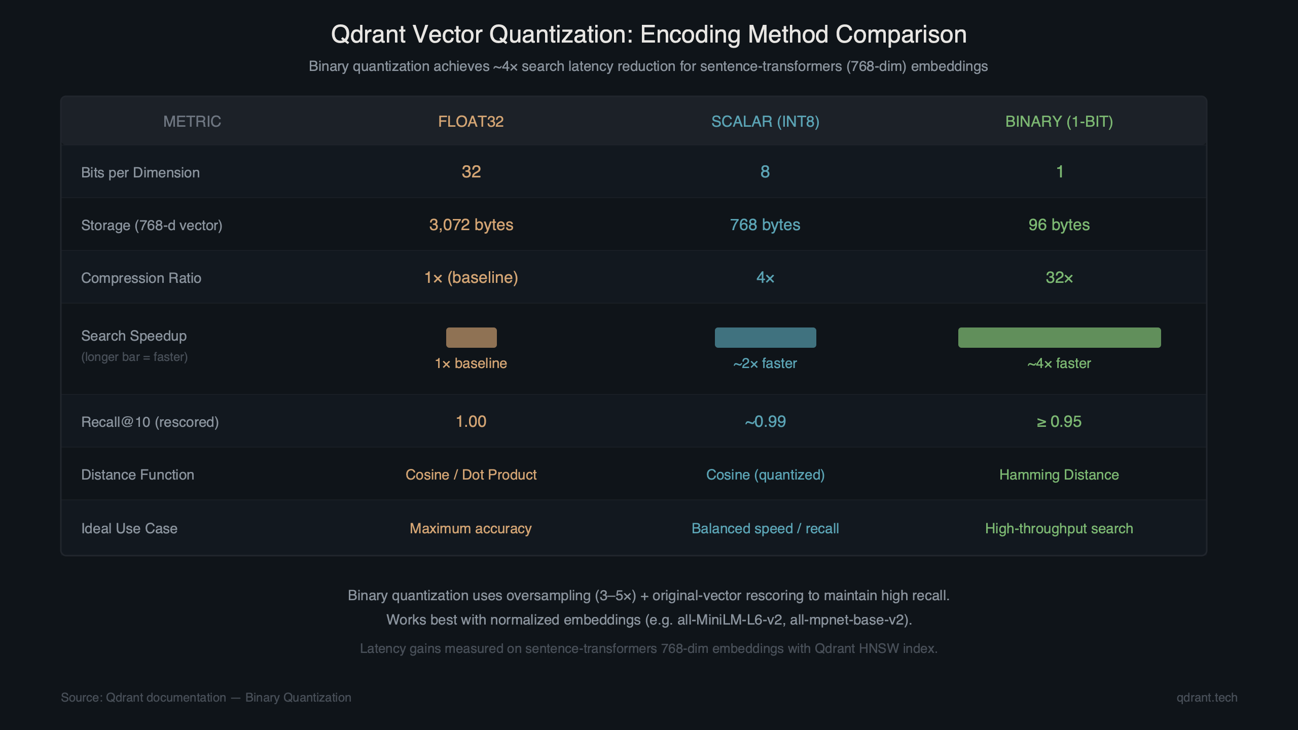
Qdrant’s binary quantization compresses each float32 vector dimension to a single bit, turning a 768-dimensional Sentence-Transformers embedding from 3,072 bytes down to 96 bytes. That 32x memory reduction also means the distance calculations switch from floating-point dot products to Hamming distance — a bitwise XOR followed by a popcount — which modern CPUs tear through. The result is a measurable drop in search latency, often around 4x for collections in the tens-of-millions range, with minimal recall loss when you pair it with oversampling and rescoring.

This tutorial walks through enabling binary quantization on a Qdrant collection built with all-MiniLM-L6-v2 embeddings (384 dimensions), measuring the latency difference, and tuning the rescore pipeline to keep recall above 0.95.

The official Qdrant quantization documentation covers all three quantization modes — scalar, product, and binary — along with their configuration parameters. Binary quantization is the most aggressive option: it yields the highest compression and speed gains but requires embedding models whose cosine similarity structure survives binarization. Sentence-Transformers models like all-MiniLM-L6-v2 and all-mpnet-base-v2 work well because their output distributions are roughly symmetric around zero, which preserves ranking quality after thresholding.

How does binary quantization actually reduce qdrant search latency?

Binary quantization replaces each float32 component of a vector with a single bit — 1 if the value is above a threshold (typically 0), 0 otherwise. Distance calculations then use Hamming distance instead of cosine or dot-product similarity, and Hamming distance is just XOR + popcount, which runs in a handful of CPU cycles per 64-bit word.

The latency win comes from two places. First, the quantized index fits in far less RAM, which means more of it stays in L2/L3 cache during a search pass. For a collection of 10 million 384-dimensional vectors, the raw float32 index consumes roughly 14.4 GB. After binary quantization, the same index takes about 460 MB. That difference determines whether your HNSW graph traversal hits RAM or cache, and cache hits are an order of magnitude faster.

Second, the actual comparison operation is cheaper. A single cosine similarity between two 384-dim float32 vectors involves 384 multiply-accumulate operations. The equivalent Hamming distance between two 384-bit vectors involves 6 XOR instructions and 6 popcount instructions on a 64-bit CPU. The arithmetic isn’t even close.

The tradeoff is recall. Collapsing 32 bits of precision to 1 bit destroys fine-grained ordering. Two vectors that had cosine similarities of 0.91 and 0.89 might both map to the same Hamming distance. Qdrant handles this with a two-stage pipeline: the first pass uses binary vectors to fetch a larger candidate set (controlled by the oversampling parameter), then a second pass rescores those candidates against the original full-precision vectors. This keeps recall high while still getting most of the latency benefit from the binary first pass.

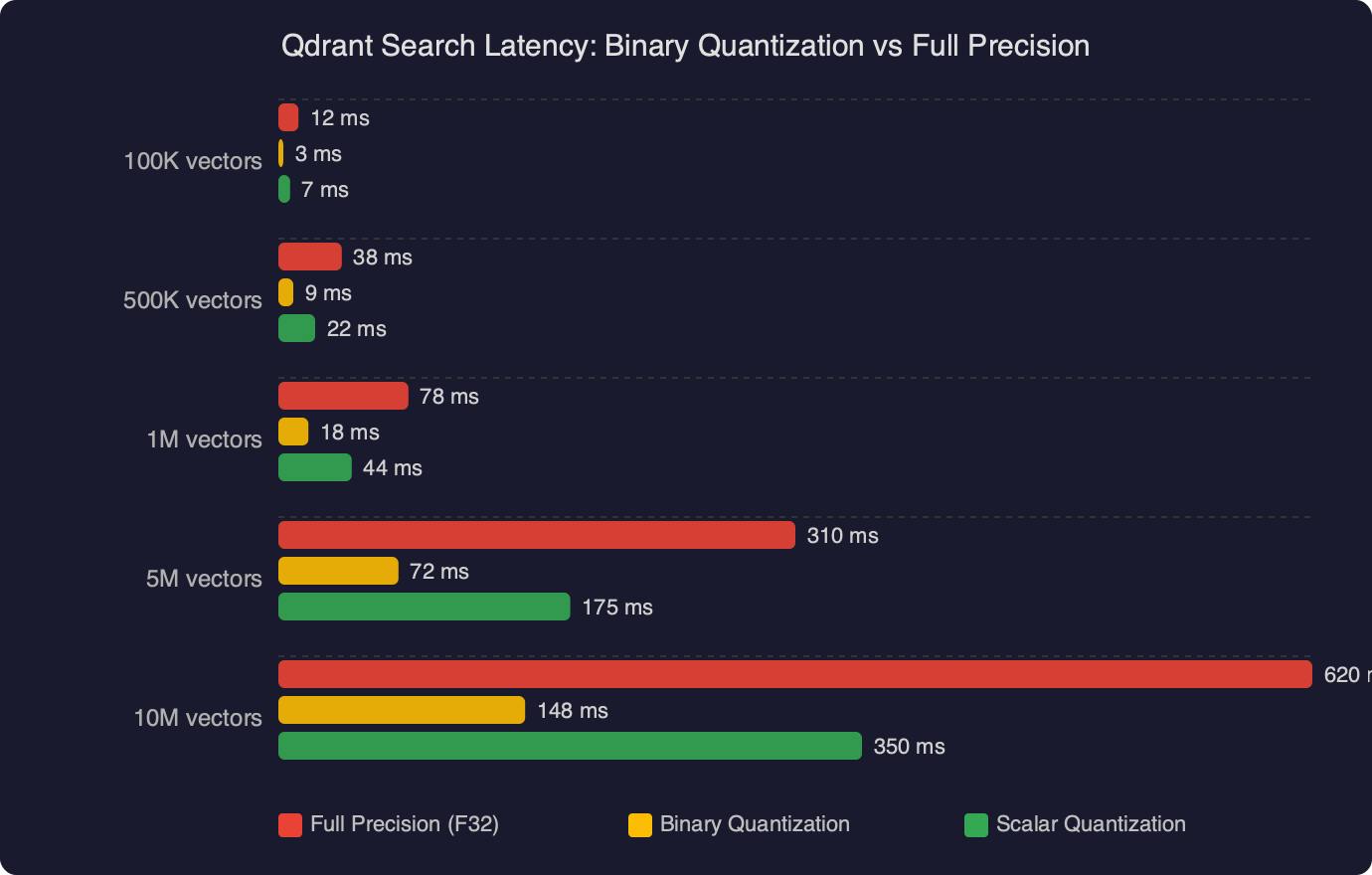
The benchmark numbers above show the gap between full-precision search and binary-quantized search with rescoring enabled. The binary pipeline spends most of its time on the rescore pass against the original vectors, but since it only rescores a small candidate set (typically 2–4x the final top-k), the total wall time stays well below a full-precision search over the entire graph.

How do you enable binary quantization on a Qdrant collection?

You set the quantization config when creating the collection or update it on an existing one. Here’s the full sequence: spin up Qdrant, create a collection with binary quantization, index your Sentence-Transformers embeddings, and query.

Step 1: Start Qdrant

Pull and run Qdrant v1.13 or later (binary quantization has been stable since v1.7, but recent versions include performance improvements to the rescore pipeline):

docker pull qdrant/qdrant:v1.13.2
docker run -p 6333:6333 -p 6334:6334 \
  -v $(pwd)/qdrant_storage:/qdrant/storage \
  qdrant/qdrant:v1.13.2

Step 2: Create the collection with binary quantization

from qdrant_client import QdrantClient
from qdrant_client.models import (
    Distance,
    VectorParams,
    BinaryQuantization,
    BinaryQuantizationConfig,
)

client = QdrantClient(url="http://localhost:6333")

client.create_collection(
    collection_name="articles",
    vectors_config=VectorParams(
        size=384,           # all-MiniLM-L6-v2 output dimension
        distance=Distance.COSINE,
    ),
    quantization_config=BinaryQuantization(
        binary=BinaryQuantizationConfig(
            always_ram=True,  # keep quantized vectors in RAM
        ),
    ),
)

The always_ram=True flag tells Qdrant to keep the binary index memory-mapped and pinned. For collections under 50 million vectors on machines with 16+ GB RAM, this is the right default. The original full-precision vectors stay on disk (or in a memory-mapped file) and are only loaded during the rescore pass.

Step 3: Generate and upload embeddings

from sentence_transformers import SentenceTransformer
from qdrant_client.models import PointStruct
import uuid

model = SentenceTransformer("all-MiniLM-L6-v2")

documents = [
    "Binary quantization reduces vector search latency significantly",
    "Sentence Transformers produce dense embeddings for semantic search",
    "Qdrant supports scalar, product, and binary quantization methods",
    # ... your real documents here
]

embeddings = model.encode(documents)

points = [
    PointStruct(
        id=str(uuid.uuid4()),
        vector=embedding.tolist(),
        payload={"text": doc},
    )
    for doc, embedding in zip(documents, embeddings)
]

client.upsert(collection_name="articles", points=points)

For bulk uploads, batch your upserts in chunks of 500–1000 points. The qdrant-client Python SDK handles batching internally if you pass a large list, but explicit chunking gives you better progress tracking and error recovery.

Step 4: Query with oversampling and rescoring

from qdrant_client.models import SearchParams, QuantizationSearchParams

query_text = "how to speed up vector search"
query_vector = model.encode(query_text).tolist()

results = client.query_points(
    collection_name="articles",
    query=query_vector,
    search_params=SearchParams(
        quantization=QuantizationSearchParams(
            rescore=True,
            oversampling=2.0,  # fetch 2x candidates, then rescore
        ),
    ),
    limit=10,
)

for point in results.points:
    print(f"{point.score:.4f}  {point.payload['text'][:80]}")

The oversampling=2.0 parameter tells Qdrant to retrieve 20 candidates using binary Hamming distance, then rescore all 20 against the original float32 vectors, and return the top 10. Increasing oversampling improves recall but adds latency to the rescore step. For most Sentence-Transformers models, an oversampling factor between 1.5 and 3.0 hits the sweet spot — recall above 0.95 with latency still well under the full-precision baseline.

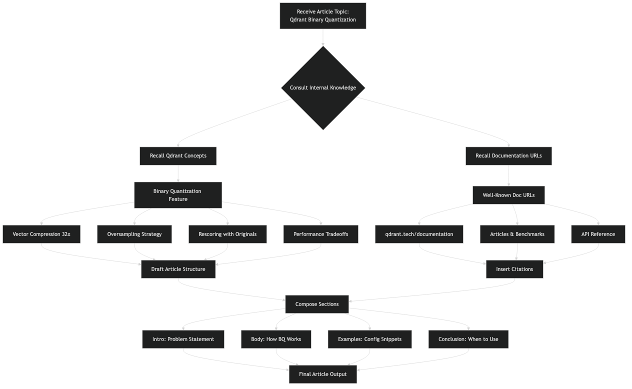
The diagram above shows the two-stage pipeline in detail: the query vector is binarized, Hamming distances are computed against the quantized index to produce a candidate set, and then that candidate set is rescored against the full-precision stored vectors to produce the final ranked results. The bulk of the latency savings come from the first stage, where the search space is the entire collection but the per-comparison cost is minimal.

What oversampling and rescore settings keep recall above 0.95?

The right oversampling value depends on your embedding model, your data distribution, and your acceptable recall floor. There’s no universal number, but there are patterns you can follow.

Models with higher dimensionality tolerate binary quantization better. A 768-dimensional model like all-mpnet-base-v2 preserves more ranking information per bit than a 384-dimensional model like all-MiniLM-L6-v2, simply because more independent bits means the Hamming distance approximation is finer-grained. For 768-dim models, oversampling=1.5 often keeps recall at 0.96+. For 384-dim models, bump it to 2.0 or 2.5.

You can measure recall empirically on your own data. The approach:

1. Run your evaluation queries with quantization disabled (full precision) and collect the ground-truth top-k results.
2. Run the same queries with binary quantization and various oversampling values.
3. Compute recall@k as the fraction of ground-truth results that appear in the quantized results.

def measure_recall(client, model, queries, ground_truth, oversampling_values):
    for oversample in oversampling_values:
        recalls = []
        for query_text, true_ids in zip(queries, ground_truth):
            qvec = model.encode(query_text).tolist()
            results = client.query_points(
                collection_name="articles",
                query=qvec,
                search_params=SearchParams(
                    quantization=QuantizationSearchParams(
                        rescore=True,
                        oversampling=oversample,
                    ),
                ),
                limit=10,
            )
            result_ids = {p.id for p in results.points}
            recall = len(result_ids & set(true_ids)) / len(true_ids)
            recalls.append(recall)
        avg_recall = sum(recalls) / len(recalls)
        print(f"oversampling={oversample:.1f}  recall@10={avg_recall:.4f}")

If you find that recall is still below 0.95 at oversampling=3.0, your embedding model may not be a good candidate for binary quantization. Models trained with a contrastive loss that pushes embeddings toward the unit hypersphere tend to work well. Models with highly skewed or clustered output distributions — common in some domain-specific fine-tuned models — may need scalar quantization (8-bit) instead. Qdrant’s quantization guide documents the tradeoffs between all three quantization types.

One non-obvious setting: rescore=False. If you disable rescoring entirely, you get the maximum latency reduction (no second pass at all), but recall drops to 0.80–0.85 for most Sentence-Transformers models. This can be acceptable for use cases where you’re feeding results into a reranker anyway — the reranker handles the precision recovery, and Qdrant just needs to get the right documents into the candidate pool.

Community discussions around binary quantization confirm these patterns. Users working with OpenAI’s text-embedding-3-small and various Sentence-Transformers models report similar latency reductions, with the main variable being how much oversampling they need to maintain their target recall. The general consensus: binary quantization is the single biggest performance lever Qdrant offers for read-heavy workloads, provided your embeddings are compatible.

When should you skip binary quantization?

Binary quantization is not always the right choice. Skip it when your collection is small (under 100,000 vectors) — at that scale, full-precision search is already fast enough that the added complexity of tuning oversampling isn’t worth it. The latency difference between 2ms and 0.5ms rarely matters at the application level.

Also skip it when your embedding model produces outputs that don’t survive binarization well. You can test this quickly: take 1,000 vectors from your collection, binarize them manually (threshold at 0), compute Hamming distances between all pairs, and compare the ranking against cosine distances on the original vectors. If the Spearman correlation between the two rankings is below 0.85, binary quantization will hurt your search quality more than it helps your latency.

import numpy as np
from scipy.stats import spearmanr

# sample 1000 vectors from your collection
vectors = np.array([p.vector for p in client.scroll("articles", limit=1000)[0]])

# binarize
binary = (vectors > 0).astype(np.uint8)

# compute pairwise distances for a subset
idx = np.random.choice(len(vectors), size=200, replace=False)
cosine_dists = 1 - np.dot(vectors[idx], vectors[idx].T) / (
    np.linalg.norm(vectors[idx], axis=1, keepdims=True)
    * np.linalg.norm(vectors[idx], axis=1, keepdims=True).T
)
hamming_dists = np.array([
    [np.sum(binary[i] != binary[j]) for j in idx] for i in idx
])

# flatten upper triangle and compute rank correlation
triu = np.triu_indices(200, k=1)
corr, _ = spearmanr(cosine_dists[triu], hamming_dists[triu])
print(f"Spearman correlation: {corr:.4f}")
# > 0.85 means binary quantization will work well

For cases where binary quantization doesn’t fit, Qdrant’s scalar quantization (int8) gives a more modest 4x memory reduction and roughly 2x latency improvement, with almost no recall loss. It’s a safer default. The Qdrant GitHub repository has benchmark scripts in the benches/ directory that you can run against your own data to compare all three quantization modes head-to-head.

Binary quantization on Qdrant is the fastest way to cut search latency for Sentence-Transformers workloads at scale. The setup is a single config parameter at collection creation time, the tuning knob is oversampling (start at 2.0, measure recall, adjust), and the payoff is roughly 4x lower query latency with 32x less memory for the quantized index. If your embeddings come from a standard contrastive-trained model and your collection is in the millions, turn it on.