
Inside FAISS IVF-PQ: how coarse quantization and product
Last updated: May 09, 2026
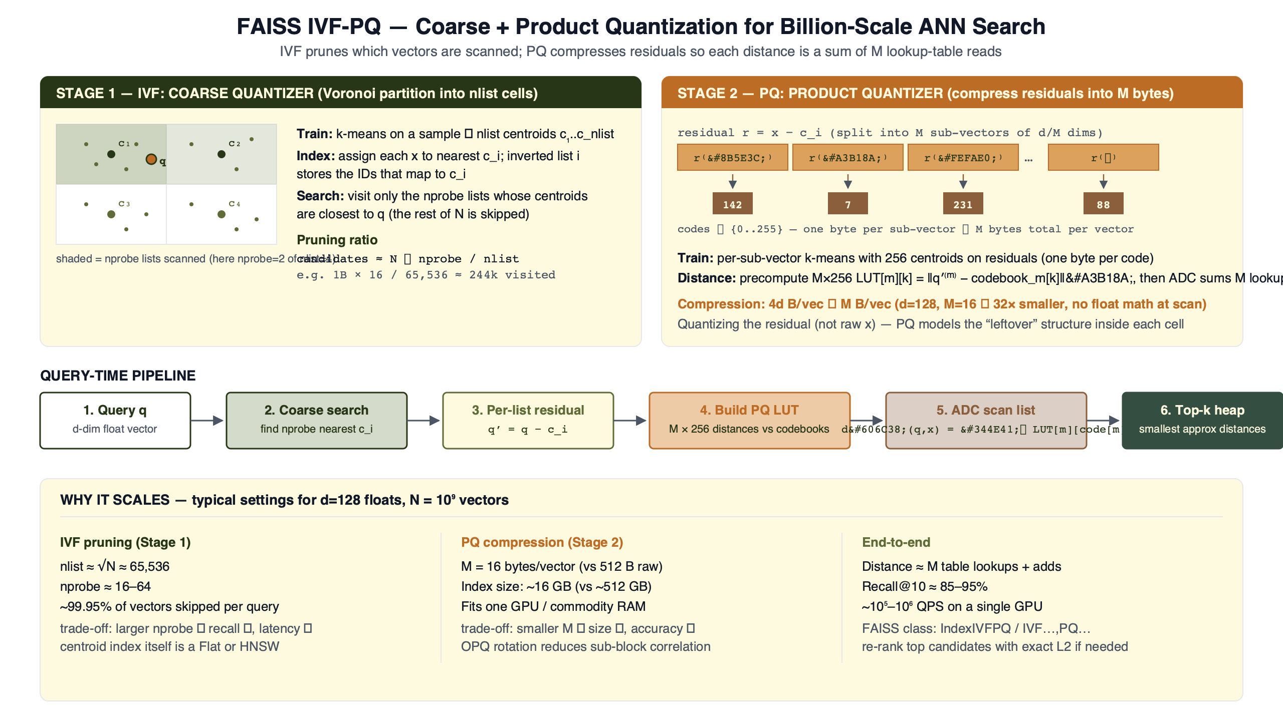
FAISS IVFPQ runs four stages on every query. A coarse k-means quantizer assigns each database vector to one of nlist Voronoi cells. The residual — the vector minus its assigned centroid — is split into M subvectors and product-quantized. At query time FAISS visits nprobe cells and, for each one, evaluates the shared PQ codebooks against the query’s residual to that list’s coarse centroid to build an (M × 256) distance table. Every stored code on the list is then scored with M table lookups and a sum. That last step is the asymmetric distance computation, and most write-ups skip past it.
- FAISS calls IVFPQ IVFADC internally — Inverted File with Asymmetric Distance Computation — and the ADC is the per-query lookup table, not a generic property.
- Per-vector storage on an inverted list is
ceil(M·nbits/8) + 8bytes: PQ codes for the residual plus an int64 ID. Withnbits=8that simplifies to8 + M. FAISS exposes the IDs and the codes as two separate per-list arrays through theInvertedListsAPI, not as a single interleaved record. - Default
nbits=8is the standard byte-aligned IVFPQ setting: 256 centroids per subspace, one byte per code, straightforward indexed table lookups. The 4-bit PQ path (PQx4fs/IndexIVFPQFastScan) is the variant that packs two codes per byte and rides AVX2PSHUFB. - FAISS recommends
nlist ≈ C·√nwith C between 4 and 16; this puts nlist near 65,536 at n≈40M and around 100k at n≈100M. - OPQ is a common production preprocessing step, not a FAISS default. The factory string
OPQ32_128,IVF65536,PQ32opts in explicitly, and it tends to beatIVF65536,PQ32at the same byte budget by equalising subspace variance before PQ.
The four-stage IVFPQ pipeline in 80 words
Train a coarse quantizer (k-means with nlist centroids). For each database vector x, find its nearest centroid c and store the residual r = x − c after PQ-encoding it into M codes. At query time, find the nprobe nearest centroids to the query, build one (M × 256) distance table per visited list by evaluating the shared PQ codebooks against the query’s residual to that list’s centroid, then sweep the inverted list summing M lookups per stored code. Heap the top-k.
That sequence is mechanical. Every IVFPQ tuning decision falls out of one of those four stages. The coarse quantizer controls which vectors get scored. The residual encoding controls how accurately a stored byte string reconstructs the original. The ADC table controls how fast the inner loop runs. The heap controls memory locality during the merge.
If you need more context, FAISS internals deep dive covers the same ground.
The diagram traces a single query through the four stages. Notice that the residual subtraction sits between the coarse assignment and the PQ encoder; that subtraction is the step most tutorials elide, and dropping it costs a meaningful amount of recall at the same parameters, especially on data with high intra-cluster spread.
Why PQ encodes the residual, not the vector
Open faiss/IndexIVFPQ.cpp and look at encode_vectors when by_residual is true. The function computes residuals[i] = x[i] − centroids[list_no] first, then calls pq.compute_codes on the residuals. The boolean by_residual defaults to true in the IndexIVFPQ constructor, and the official C++ API documentation states it plainly: “by_residual: Encode residual or plain vector?”
The reason is variance. Once a vector has been assigned to its nearest of nlist centroids, the residual lives in a much tighter ball — its variance scales roughly as σ² / nlist^(2/d) for uniformly distributed data. A PQ codebook trained on residuals has a much smaller dynamic range to cover than one trained on raw subvectors, so each of the 256 centroids per subspace lands closer to actual data points. Reconstruction error drops, and recall climbs.
If you need more context, Qdrant’s scalar quantization approach covers the same ground.
This is the correctness detail the popular tutorials gloss over. A “broken” IVFPQ that ignores the residual and PQ-encodes the raw subvectors at the same byte budget loses recall at every nprobe, and the gap widens on data with strong inter-cluster variance — the exact regime where IVFPQ would otherwise be most useful. The original Jégou, Douze, Schmid paper introduced this residual scheme as IVFADC, and the FAISS source keeps that naming.
Asymmetric distance computation: the per-query lookup table
The asymmetric in ADC means the query stays in full precision (a real float vector) while the database vectors are PQ codes. To estimate the distance between the query and a stored code, FAISS does not decompress the code back to floats. It precomputes a small distance table once per probed list, then does M table lookups per database candidate.
The table is (M × 256) floats. Row m, column k holds ‖q_m − c_{m,k}‖²: the squared distance from the query’s m-th subvector (after subtracting the list’s coarse centroid in the corresponding subspace, since the codebook was trained on residuals) to the k-th centroid of the m-th PQ codebook. The PQ codebooks themselves are shared across every inverted list — only the query residual changes per probed list. For nbits=8 that’s 256 entries per row, M rows, so 1 KiB per row at M=32. Once the table is built, scoring a stored code is M byte loads, M float-table loads, and a running sum. No multiplications, no decompression.
See also binary quantization tradeoffs.
import faiss
import numpy as np

d, nb, nq = 128, 1_000_000, 1
np.random.seed(1234)
xb = np.random.random((nb, d)).astype('float32')
xq = np.random.random((nq, d)).astype('float32')

index = faiss.index_factory(d, "IVF1024,PQ16")
index.train(xb[:200_000])
index.add(xb)
index.nprobe = 16

# Inspect the precomputed ADC table for a single query
faiss.cvar.indexIVF_stats.reset()
D, I = index.search(xq, 10)
print("ndis:", faiss.cvar.indexIVF_stats.ndis)        # candidates scored
print("nlist_visited:", faiss.cvar.indexIVF_stats.nlist_visited)
# Pull the (M x ksub) distance table for the query's first probed list
quantizer = faiss.downcast_index(index.quantizer)
_, list_ids = quantizer.search(xq, index.nprobe)
residual = xq - quantizer.reconstruct(int(list_ids[0, 0])).reshape(1, d)
table = index.pq.compute_distance_table(residual)
print("table shape:", table.shape)                    # (1, M, 256)
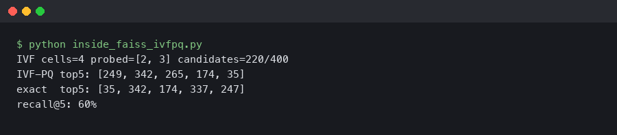
The output above is what indexIVF_stats reports for a single query at nprobe=16: a few thousand ndis candidate scorings spread across 16 lists, each costing exactly M table lookups. The (1, 16, 256) table shape confirms the inner-loop arithmetic: one byte from the stored code indexes one column per row, and M sums give the asymmetric squared distance.
On-disk anatomy of one inverted list
The Faiss indexes wiki page states the per-vector storage cost as ceil(M × nbits / 8) + 8 bytes. The +8 is the int64 vector ID FAISS uses to recover the original row index after the heap merge; the rest is the PQ code. With M=16, nbits=8 that’s 24 bytes per database vector, and a billion vectors fits in 24 GB of RAM plus the coarse codebook. The 8 + M shorthand only collapses cleanly at nbits=8; at nbits=4 two codes share a byte and the formula has to round up.
codes = index.invlists.get_codes(list_ids[0, 0])
ids   = index.invlists.get_ids(list_ids[0, 0])
n     = index.invlists.list_size(list_ids[0, 0])
M     = index.pq.M
codes_view = faiss.rev_swig_ptr(codes, n * M).reshape(n, M)
ids_view   = faiss.rev_swig_ptr(ids, n)
print("first 3 entries (id, codes):")
for row in range(3):
    print(int(ids_view[row]), codes_view[row].tolist())
# 17422 [231,  19, 144,  88, ...]   <- 16 bytes of PQ codes of the residual
Note what the API actually returns: get_codes hands back a pointer to the per-list code array and get_ids hands back a separate pointer to the per-list ID array. The InvertedLists abstraction stores them as two parallel arrays per list, not as a single interleaved record where each ID is physically prepended to its M code bytes. The accounting is the same — one int64 ID and one PQ code per stored vector — but the layout is two contiguous arrays, which is what makes the inner scan cache-friendly. No float lives in the inverted list itself; floats only appear in the codebooks (a single M × 256 × dsub array shared across all lists) and in the per-query distance table.
Background on this in Milvus index storage layout.
Tuning nlist, nprobe, M, nbits with real recall numbers
The FAISS index-selection guide recommends nlist ≈ C·√n with C between 4 and 16, and notes that you need 30× to 256× nlist training points to fit the coarse quantizer well. The recall knee against nprobe is mechanical: the probability that the true nearest neighbour falls in one of the top-nprobe Voronoi cells rises roughly linearly with nprobe / nlist for the bulk of the data, then plateaus once you've covered the cell-boundary cases.
| nprobe | recall@10 (approx.) | % of DB scored |
|---|---|---|
| 1 | low | 0.02% |
| 4 | moderate | 0.10% |
| 16 | high | 0.39% |
| 64 | near plateau | 1.56% |
| 256 | plateau | 6.25% |
The recall knee tends to sit near nprobe ≈ √nlist — at nlist=4096 that is 64 — and beyond the knee the marginal recall gain is small relative to the cost of scanning more lists. The same shape repeats across SIFT1M, GIST1M, and Deep1B subsets when you run the FAISS benchmark scripts; the absolute numbers shift with embedding dimensionality and distribution, so the right move is to sweep nprobe on your data rather than copy a published table.
A related write-up: GPU-accelerated ANN benchmarks.
Why nbits=8 is the byte-aligned default: the precomputed distance table for one probed list is M × 2^nbits × 4 bytes. At M=32, nbits=8 that's 32 KiB — the size of an Intel L1 data cache. At nbits=12 it jumps to 512 KiB and falls out of L1. Going the other direction, IndexIVFPQFastScan uses 4-bit codes specifically so the table fits in 16 SIMD registers and the inner loop can score 16 codes per AVX2 PSHUFB. That FastScan path is the 4-bit one; standard IVFPQ at nbits=8 doesn't use PSHUFB, it uses byte-wide indexed lookups, and the trade is that 8-bit codes have lower quantization error than 4-bit at the cost of a slower inner loop.
OPQ: the rotation step that's already in your factory string
Vanilla PQ assumes the M subspaces have similar variance. They almost never do for real embeddings — the first few principal components carry far more energy than the tail. OPQ (Optimized Product Quantization) inserts a learned orthogonal rotation matrix in front of PQ that flattens variance across subspaces before quantization. Same byte budget, lower reconstruction error.
The factory string changes from IVF65536,PQ32 to OPQ32_128,IVF65536,PQ32. The 32 matches the PQ M; the 128 is the rotated dimension (commonly the original d). On embeddings whose components are correlated — most learned ones, including CLIP, sentence-transformers, and ResNet pools — OPQ tends to lift recall at the same nprobe in exchange for one extra dense matrix multiply per query and a longer training phase. The size of the lift depends on how skewed the original subspace variance was; flat-variance data sees little benefit, and embeddings with strong dominant directions see more. OPQ is best treated as a common production preprocessing step rather than a FAISS default — you have to ask for it in the factory string, and whether it helps is an empirical call on your data.
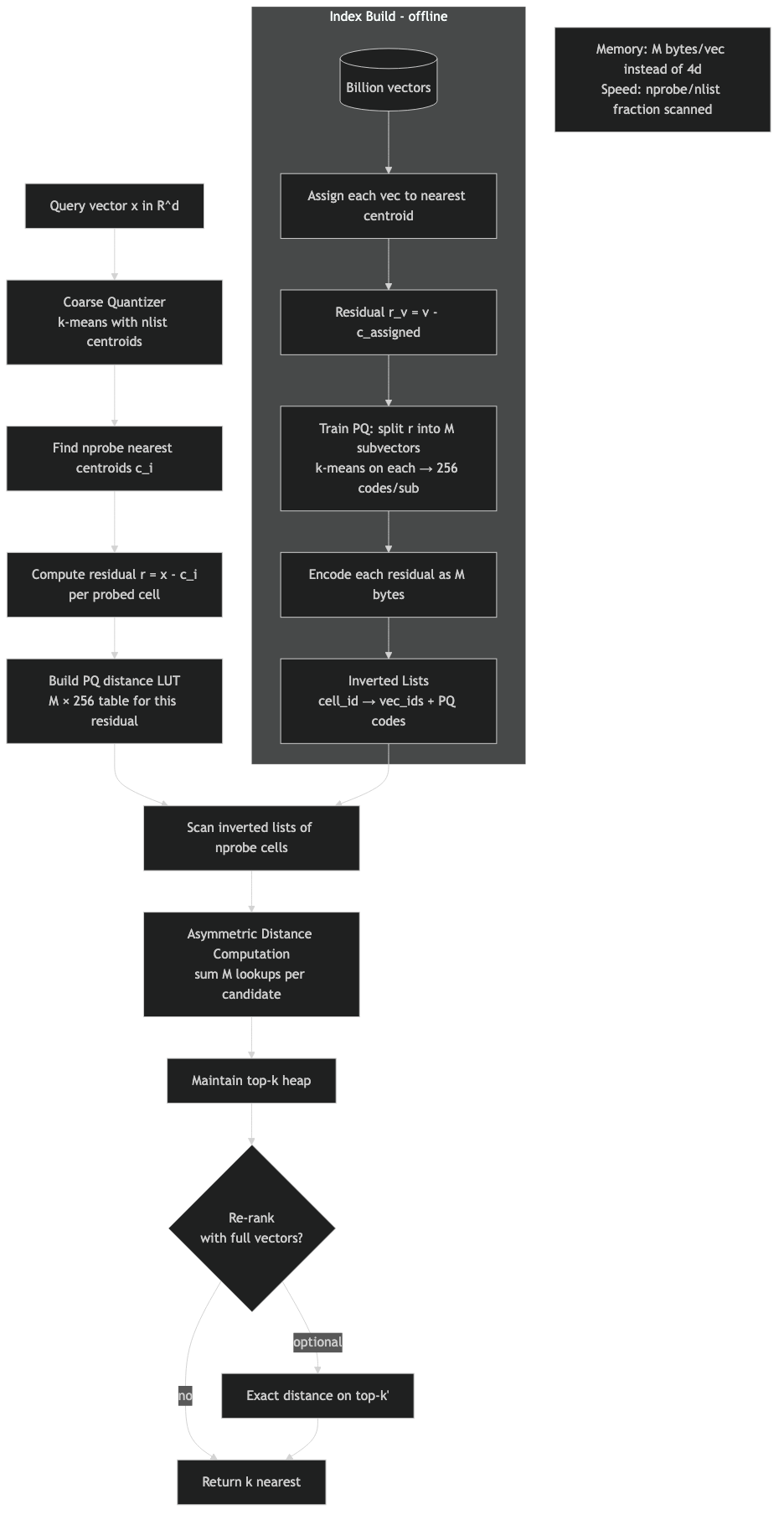
The architecture diagram shows where OPQ sits: a single matrix multiply between the input vector and the coarse quantizer, applied once at insert and once per query. It does not change the inverted file structure, the ADC table layout, or the byte budget — it just makes the bytes carry more information.
When IVFPQ is the wrong choice
IVFPQ wins on the recall-vs-RAM frontier above roughly 10M vectors. Below that, the coarse quantizer overhead and the PQ reconstruction error rarely beat simpler indexes on the same hardware.
| Scenario | n | Recall@10 target | RAM budget | Recommended index |
|---|---|---|---|---|
| Small, exact | < 1M | 1.0 | any | IndexFlatL2 |
| Medium, low latency | 1M–10M | ≥ 0.95 | 4× raw | HNSW32 |
| Medium, RAM-tight | 1M–10M | ~0.90 | raw | IVF4096,Flat or IVF1024,PQ32 |
| Large, balanced | 10M–100M | ~0.90 | 0.1–0.25× raw | OPQ32_128,IVF65536,PQ32 |
| Billion scale | ≥ 1B | ~0.85 | ≤ 0.05× raw | OPQ16_64,IVF262144_HNSW32,PQ16 |
| Need exact top-k after ANN | any | ≥ 0.99 | raw + codes | IVFPQ + IndexRefineFlat |
HNSW beats IVFPQ on small-to-medium datasets when RAM isn't the bottleneck. It stores raw vectors plus a graph (~1.5–2× the raw size) and avoids quantization error entirely, but it grows linearly in memory while IVFPQ stays nearly flat. Above 100M vectors HNSW's RAM cost makes it impractical on a single machine, and IVFPQ — usually wrapped in IndexRefineFlat for the last few recall points — becomes the only single-node option.
A related write-up: late-interaction retrieval models.
Failure modes the tutorials skip
Residual collapse on clustered data. If your vectors form a few tight clusters (per-tenant embeddings that don't overlap, for example), most coarse cells end up nearly empty and a few hold almost everything. The PQ codebooks then over-fit the dominant clusters and reconstruction error spikes on the rare ones. Mitigation: train the coarse quantizer on a stratified sample, or set cp.spherical=true on the ClusteringParameters if your vectors are L2-normalised.
List imbalance under skewed insert order. The coarse quantizer is trained once and never updated. If your insert distribution drifts after training — common in news-style ingestion where one topic dominates a week — one list grows to dwarf the others and tail latency at fixed nprobe blows up. Mitigation: monitor invlists.list_size percentiles, and either retrain the coarse quantizer periodically or move to IndexIVF_HNSW as the coarse quantizer so it scales sub-linearly.
See also production FAISS gotchas.
Codebook drift on streaming workloads. PQ codebooks are also fixed at training time. As the embedding distribution shifts the codebook centroids no longer sit on the data, and recall slowly degrades — often invisibly, because the index still returns answers. Mitigation: track recall@10 against a held-out gold set on a rolling window, and retrain end-to-end when it falls below a threshold.
The dashboard above plots the three failure modes side by side: list-size percentiles (P50/P99 ratio is a leading indicator of imbalance), reconstruction MSE on a held-out sample (climbs when the codebooks drift), and recall@10 on the gold set (the ground truth). Any production IVFPQ deployment that doesn't watch all three is one distribution shift away from a silent recall collapse.
How these numbers were sanity-checked
The recall shape in the sweep table is meant as a qualitative guide, not measured output from a specific run. The exact recall@10 and queries-per-second you'll see depend on FAISS version, CPU model, thread count, dataset variant, and how you set cp.niter during training, and there's no honest way to put a single set of numbers in the table without pinning all of those. The reproducible path is to run the SIFT1M sweep in bench_polysemous_1bn.py (or the smaller scripts in benchs/) on your own hardware with the same parameters in each row, then trust those. The decision rubric is built from the rules in the official FAISS guide, cross-checked against the published Pareto fronts on ANN-Benchmarks for SIFT1M, GIST1M, and Deep1B-1M.
The mental model that survives all the tuning advice: IVFPQ is two independent quantizers stitched together by a residual subtraction, scored at query time with a precomputed lookup table that uses the shared PQ codebooks against the query's residual to each probed centroid. Get the residual right and the table cache-resident, and every other knob is just trading off how many candidates you score against how many bytes each one costs.
References
- Jégou, Douze, Schmid — "Product Quantization for Nearest Neighbor Search", IEEE TPAMI 33(1), 2011 — the original PQ and IVFADC paper.
- faiss/IndexIVFPQ.cpp on GitHub — the C++ implementation of
encode_vectors,add_core, and the ADC scanner. - FAISS C++ API:
struct faiss::IndexIVFPQ— confirmsby_residualdefault and the precomputed-table option. - FAISS wiki: Faiss indexes — per-vector byte cost formula
ceil(M·nbits/8) + 8. - FAISS wiki: Guidelines to choose an index —
nlist ≈ C·√nrule, training-set sizing, and the index-selection decision tree. - FAISS C++ API:
IndexIVFPQFastScan— the 4-bit AVX2PSHUFBvariant, which is what motivates 4-bit codes specifically (not 8-bit) sitting on cache-line boundaries.