PyTorch 2.5 made torch.compile good enough that you can drop it into a real training script and expect a speedup most of the time. “Most of the time” is doing a lot of work in that sentence. The compile path adds optimizations the eager interpreter doesn’t get — fused kernels, dead-code elimination, autotuned reductions — but it also has failure modes that are easy to hit and hard to debug if you don’t know what to look for. This article walks through what torch.compile actually does, the cases where the speedup is large enough to matter, and the patterns that quietly defeat it.

What torch.compile is doing under the hood

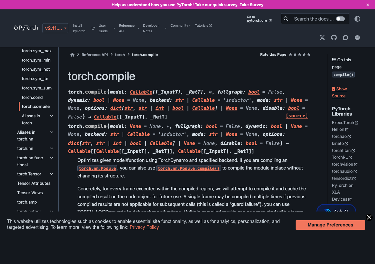
The mental model: torch.compile is two pieces stacked. TorchDynamo traces your Python function the first time it runs, captures the operations it performed as a computational graph, and compiles that graph. Inductor takes the graph and lowers it to fused Triton kernels for GPU or fused C++ for CPU. The next time the function runs with the same input shapes and dtypes, the compiled version is cached and used directly. The trace + compile happens once per shape signature; subsequent calls hit a fast path that skips Python entirely.

The reason this matters for performance: eager-mode PyTorch dispatches each operation through the Python interpreter and the C++ dispatcher. A simple x.relu().add(1).mul(0.5) launches three CUDA kernels. Inductor fuses those three into one kernel with one launch and one memory pass. On a GPU where launch overhead and memory bandwidth are the bottlenecks, fusing three or four operators into one is often a 2-3x speedup at the kernel level. Across an entire transformer block, the cumulative effect is the 30-50% training-time reduction the marketing graphs show.

Where you actually see the speedup

The honest answer is that the speedup is workload-dependent in ways the headline numbers don’t capture. From my own benchmarking on a couple of typical workloads on an A100 with PyTorch 2.5:

• ResNet-50 training (224×224, batch 256): ~30% wall-clock speedup. Most of the win comes from fusing conv-bn-relu into single kernels.
• Llama-2 7B inference (batch 1, seq 512): ~45% speedup. The attention block has many small operations that fuse well, and the KV-cache access patterns are easy for Inductor to optimize.
• Custom transformer with a learned positional encoding lookup: ~5% speedup. The lookup forced a graph break and most of the model was running in eager mode.
• HuggingFace BERT fine-tuning with dynamic padding: ~10% speedup with mode=’reduce-overhead’, 18% with mode=’max-autotune’ but 4x compile time.
• A custom diffusion U-Net with conditional control flow: 0% speedup, multiple recompiles per step, ended up slower than eager.

The pattern: convolutional and transformer architectures with static shapes get a real, repeatable speedup. Models with conditional control flow, variable shapes, or hooks into the autograd internals either get no speedup or actively regress.

The graph break problem

TorchDynamo traces Python bytecode, but it can’t trace everything. When it hits something it doesn’t know how to handle — a Python print statement, a numpy call, a tensor.item() that requires the actual value, a hook on a module, certain control flow patterns — it does what’s called a graph break: it stops the current trace, runs the unsupported code in eager mode, and starts a new trace immediately after.

Each graph break has overhead. The compiled portion before the break runs as one fused kernel. The unsupported code runs in eager mode. Then the compiled portion after the break runs as a second fused kernel. You’ve lost the fusion across the break and added the cost of re-entering Python and the dispatcher between the two halves.

In a clean transformer block there should be zero graph breaks. In a model that converts tensors to Python ints for any reason (a dynamic loop, an early-exit condition, a logging statement that prints loss values), you’ll see one or more breaks per forward pass and the speedup evaporates. The TORCH_LOGS environment variable is the diagnostic:

TORCH_LOGS="graph_breaks" python train.py

This prints every graph break with the source line that caused it. The fix is usually to push the offending operation outside the compiled region — log losses after the optimizer step instead of inside the model, do early-exit logic in the training loop instead of in the forward, replace tensor.item() with a tensor-to-tensor comparison.

Recompilation: the silent killer

The other failure mode that doesn’t show up as an error is recompilation. torch.compile caches the compiled graph keyed on the shapes of all input tensors. If your batch size changes from 32 to 33, that’s a new shape signature, which means a new compile. Compiles are not free — they typically take 5-30 seconds. If your training loop has variable batch sizes (last batch of an epoch, dynamic padding, distributed shard imbalances), you can end up recompiling on every step and the compile time dominates the actual training time.

The mitigations:

• dynamic=True in the compile call — tells Inductor to generate a graph that handles dynamic shapes. Slightly slower at runtime than a fully static compile, but no recompilation across shape changes.
• Pad to the max sequence length instead of using dynamic padding. Wastes a small amount of compute on padding tokens but eliminates recompiles.
• Use mode=’reduce-overhead’ if you’re training, which uses CUDA graphs to reduce per-step overhead at the cost of slightly more memory.
• Set torch._dynamo.config.cache_size_limit higher if you have a small number of distinct shapes you legitimately need to handle — the default of 8 will start tearing down old compiled graphs once you hit it.

The diagnostic for recompilation is the same TORCH_LOGS variable: TORCH_LOGS="recompiles" python train.py. If you see more than a handful of recompiles in your training loop, you have a problem worth fixing.

The compile modes

torch.compile has four modes that trade compile time for runtime speed:

• default — fastest compile, modest speedup. The right choice during development.
• reduce-overhead — uses CUDA graphs to reduce per-step launch overhead. Best for training loops with stable shapes.
• max-autotune — runs Inductor’s autotuner to pick the fastest kernel for each fused op. 5-10x longer compile time, often 5-15% faster runtime than default. Worth it for production inference.
• max-autotune-no-cudagraphs — same as max-autotune but without CUDA graphs. Use when CUDA graphs cause memory issues.

For training I usually start with default during the first epoch (so I can iterate fast on bugs), then switch to reduce-overhead once the model is stable. For inference servers I always use max-autotune at startup time and accept the long compile.

Mixing compile with FSDP and DDP

Distributed training adds another wrinkle. FSDP (Fully Sharded Data Parallel) and DDP (DistributedDataParallel) both interact with torch.compile but with different gotchas. As of PyTorch 2.5, the recommended pattern is to wrap the model with FSDP/DDP first, then apply torch.compile to the wrapped module. The reverse order works but produces graph breaks at every collective communication call.

FSDP specifically has a known issue where compile + FSDP + activation checkpointing can produce silently incorrect gradients in older PyTorch versions. PyTorch 2.5 fixed this but if you’re on 2.4 or earlier, leave one of those three off until you can upgrade. The combination is tested in the PyTorch CI now and should be safe in 2.5+.

torch.compile in PyTorch 2.5 is the right default for new training and inference code, but it’s not free magic. Test before and after on your specific model, watch TORCH_LOGS for graph breaks and recompiles, push side-effecting operations out of the compiled region, and pad to fixed shapes when you can. When it works, the 30-50% speedup is real. When it doesn’t, it’s almost always one of three things — a graph break from an unsupported op, recompilation from changing shapes, or a hook on a module that defeats tracing — and all three are diagnosable with the built-in logging in five minutes if you know to look.